Plotting box- and chevron folds

This section describes how the default script can be easily modified to plot box and chevron folds. A variety of folds can be defined using simplified Fourier series (Stabler, C.L., 1968, Simplified Fourier analysis of fold shapes, Tectonophysics 6, 343-350.):





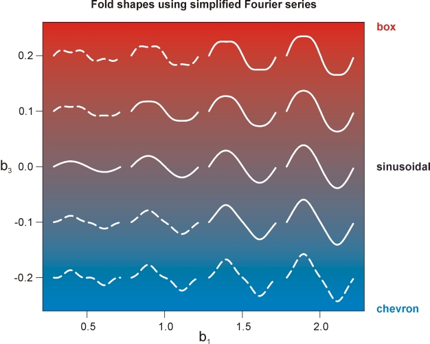
where b₁ and b₃ are Fourier coefficients that determine the fold shape and w is the wavelength. The first coefficient modifies the amplitude of the fold, whereas the third the shape (box fold if b₃ positive and chevron fold if negative). A chart of fold shapes that were plotted using the above equation is shown below with double hinged folds shown as dashed lines.



To plot box- and chevron folds and their structure contours open the file structure_contours_folds.m in Matlab. In the Matlab editor select the menu ‘debug’ and ‘run’. In the Matlab command window the following text appears:

Please choose topography

valley (enter 1), ridge (enter 2) or both (enter 3)?

Type 1, 2 or 3 and press the return key. Then the following text appears:

Please choose geological structure

Box- and Chevron folds (enter 1) or parastitc folds (enter 2)?

Type 1 and press the return key. Then the following text appears:

plunge of fold:

Type the plunge of the fold (in degrees) and press the return key. Then you are asked the following:

Please enter harmonic coefficients, b1 and b3

b1:

b3:

Type in the coefficients (some guidelines are given in the diagram above) and press return. The Matlab diagrams shown below give some examples with non-plunging (top) and 10 degree plunging box and chevron folds that were created with this script. The box fold Fourier coefficients b₁ and b₃ are 1.5 and 0.2, respectively, and chevron fold Fourier coefficients b₁ and b₃ are 1.5 and -0.1, respectively,

NEXT

BACK